Variance analysis

DISCLAIMER: Statistics is scary. To ease the stress caused by writing and reading about it, I've included cute pictures along the way. One way of making statistics less traumatizing is to use funny examples, pretty colors or banging your head with a hammer, which is probably less painful than calculating regression factors. However, if you do read this post and end up in an insane asylum, try to get the room 7. I've hidden a hammer under the pillow.
 
Statistics is the science of controlling uncertainty in measurements and estimations. It's not just about collecting data and turning it to fancy graphs, but to really ensure that the information is correct. The graphs are just the tip of the iceberg of formulaes, tests and hypotheses. This post offers short explanations on some of the basic concepts of statistics. For more information, see KhanAcademy's excellent 10-minute videos on statistics.

A completely irrelevant but cute bunny.


Statistics: A branch of mathematics dealing with the collection, analysis, interpretation, and presentation of masses of numerical data. A collection of quantitative data. A statistic would be a single term or datum in a collection of statistics, or a quantity (as the mean of a sample) that is computed from a sample.(Merriam-Webster Dictionary)

Median, mean and mode: When the numerical values of the data are arranged from smallest to largest, median is the value in the middle, or the mean of the middle values (if there are even number of results). Mean is the arithmetic mean of the values: the sum of the values divided by the number of values. Mode is the value which is represented most often in the set of data. For example, in a data set of
2  4  4  5  6  7  7  9
the median is the mean of the two values in the center ( (5+6)/2 = 5.5 ), 4 and 7 are modes and the mean is (2+4+4+5+6+7+7+9)/8 = 5.5. Note that median and mode are not always identical.

Population and sample: Population is the all past, present and future realizations of the values of the object to be measured. A population of soda cans would mean all of the cans which have been produced, are produced and will be produced in the future. Population statistics can only be estimated from a small proportion of the population, namely a sample. We select a decent amount of soda cans, measure them, and estimate how well those results might represent the whole population.

Different statistical values for a population and for a sample are sometimes calculated a bit differently. The denotations also differ. Thus it is clear when the statistics are about an observed sample or estimated for a population.

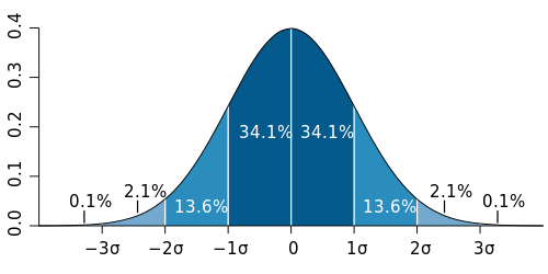
Normal distribution: The most common distribution of values, where middle-range observations are the most common, and extremely small and large observations are rare. Many natural traits, like height or IQ, are normally distributed, especially when a data set of over 30 observations is used. Normal distribution is in the shape of a Bell-curve. A really useful attribute in a normal distribution are that it's symmetrical around it's central peak:

(c) Wikipedia

Variance and standard deviation: Variance shows how far each value in the data set is from the mean.Variance is relative, and independent from the values in the data set. It doesn't measure the difference between the mean and extreme values, but the distance between them in units of standard deviation. Standard deviation is simply the square root of variance. Population variance is often denoted as sigma to the power of two (σ²), and standard deviation as sigma (σ). Sample variance is mu to the power of two (µ²), and sample standard deviation is mu (µ).

Statistical testing: Testing in statistics is rather depressing: it's about estimating the risk of being wrong. First the research hypotheses are formed, and then the actual data is collected. A  set of two or more subsamples (or subpopulations) are compared by using either parametric or non-parametric statistical tests. The aim is to estimate the risk of being wrong when the formulated H₀ (zero hypothesis) hypothesis is correct.

Variance? Is that something edible?
(c) redpandanetwork.org

H₀ is always a "nothing happens" hypothesis, and H₁ is it's opposite. Say that you've measured the weight of red pandas in two different regions in China. You calculate means, variances etc for the two samples (the two groups of pandas). Your H₀  must be that there's no difference in the weights. Your H₁ must then be either "There is difference in the weights", "the pandas in the area A are lighter" or "the pandas in the area A are heavier."




Variance analysis
 Variance analysis is a parametric test for comparing the mean of three or more subpopulations. The same comparation for two populations is done using a paired Student t-test. Variance analysis has three requirements:

1. The populations in variance analysis  must be normally distributed
2. Variances are equal in all subpopulations
3. The observations are independent (not depending on one another)

The populations may be of different size. Usually the populations in variance analysis are caused by different treatments to the studied unit. For example, pieces of meat are treated with different preservatives to find the most effective one, or the  results of different excercise programs are compared. Again the zero hypotheses is that the treatments have no effect to the results ( µ₁ = µ₂ = ... = µ_n)

The structure of variance analysis is

x_ij = µ + α_i + ε_ij

where μ = common mean
α_i = the effect of treatment i
ε_ij = random error, which is normally distributed N(0,σ)

The idea behind variance analysis is to trace the variation in the observed results into separate sources. Variation can be caused by the treatments, or by other factors (residual error). If the assumptions for variance analysis are true, residual error is normally distributed with the expected value of 0. The total variation of the observations around the mean can be divided into two sums of squares, SStreatments and SSerror. The sum of SStreatments and SSerror is SStotal. SStreatments is the sum of squares of the variation caused by the treatments. SSerror is the sum of squares of the residual error.

In the formula above,
x_ij = the j:th observation of the i:th treatment
n = number of observations in a treatment
k = number of treatments
x_i+ = sample mean in treatment i
x = sample mean of all observations


F-test
Once we've established the SStotal, it's time to use SStreatments and SSerror for estimating the population variance. The sums of squares must be divided by their degrees of freedom (df). For SStreatments df is k-1, and for SSerror it's kn-k. This gives us mean sums of squares. Finally the actual test value F is calculated:

MStreatments = SStreatments / k-1          MSerror = SSerror / nk-k

F = MStreatments / MSerror

The test value F is F-distributed with degrees of freedom k-1 and nk-k.  The larger F is, the stronger evidence it gives against the zero hypothesis. The critical values of F can be found from the F-sheet (such as this). The observed value of F is then used to find out the observed p (probability to get the observed results if H0 is true). If a test of significance gives a p-value lower than the significance level α, the null hypothesis is rejected. I.e if the observed p < chosen significance level, H0 is rejected.

More on variance analysis:
http://www.itl.nist.gov/div898/handbook/prc/section4/prc433.htm
http://www.terry.uga.edu/~pholmes/MARK5000/Classnotes2.pdf
http://en.wikipedia.org/wiki/Statistical_significance