Basics on animal genetic resources

Farm animal genetic resources, or simply AGR, refers to the genetic material we currently have in live animals and frozen in sperm banks, and which is of economical, cultural and scientific importance. Genetic diversity, both within and between breeds, is vital. Diversity

• helps the animals to adapt to their environment
• is the basis for animal breeding
• allows adaptation to changes and new breeding targets
• prevents inbreeding depression
• keeps the frequency of harmful allelels low.

Domestication has already reduced genetic diversity in farm animal species (and artifical insemination has reduced it even further). Domestication is the process by which captive animals adapt to man and the environment provided, and it is achieved through genetic changes. Genetic factors affecting domestication are inbreeding, genetic drift and selection.  

Impact of domestication on milk yield of dairy cows.

Inbreeding is necessary when selecting a desired trait, but it reduces heterozygosity and thus diversity, although it does not affect allele frequencies. Genetic drift causes alleles to become fixed or deleted randomly, and its direction cannot be estimated. Selection, both natural and artificial, has altered the fitness of certain traits. For example, in domestication species the distance to flee and fearfulness have been decreased, even though they are vital for a wild animal. These are both behavioral changes. Physiological changes involve changes in hormone levels, reproduction cycle and production traits (e.g. the increased milk yield of cows and the all-year farrowing of sows). Morphological changes have also occurred, as animals have grown larger and developed colors unseen in the wild (especially white). For an example of scientific study on domestication, see Giuffra et. al (2000) or Kantanen et al. (1999).

Studying domestication

Domestication can be studied in several methods. Paternal transmission of Y-chromosome shows traits have developed from sire to offspring. It's counterpart is the study of mtDNA (mitochondrial DNA), which is always inherited from the dam to all her offspring. mtDNA haplotypes are sequenced and aligned, and dendrograms or cladograms are drawn based on the multiple-sequence-alignment (MSA) results. The haplotypes can be further divided into groups, which helps to draw a network. For more information visit the blog The Genealogical World of Phylogenetic Networks and their post on interpreting rooted networks.

The most common method by far is still studying microsatellite markers. Usually 20-30 microsatellites are studied, but FAO has published recommendations for each animal species (FAO). Polymorphic loci with 4 or more alleles are recommended to eliminate false positives by identical-by-state -alleles. Unlike mtDNA and Y-chromosome, microsatellites are inherited from both parents to all offspring. Genotyping and aligning SNP-markers is similar to microsatellies, but requires the use of thousands or hundreds of thousands of SNP-markers. Microchip arrays are readily available for several species for SNP-analysis.

Practical application of genetic domestication studies.
(c) ILRI 2006

Studying ancestral DNA is tedious, but can yield valuable information on extinct species. Ancestral DNA can be thousands or tens of thousands of years old. It is collected either from animal remains such as fossils, teeth, wools, hides or bone pieces, or from the ground ("dirty DNA"). Ancestral DNA also helps to chart the spread of different animal and plant species and to determine temporal changes in their genetics. The problem with ancestral DNA is that the concentration of desired DNA is often low, while the concentration of microbial DNA is high. Contamination risk is very high indeed. Sterile environment must be maintained whenever possible when working with ancestral DNA. Another problem is that the ancestral DNA has been fragmented, and many chemical bonds have been broken. C > T and G > A mutations in PCR are common due to deamination. The results must be confirmed in several independent laboratories. In addition, all results derived from ancestral DNA must fit in to earlier context.

Retroviruses have been used as a study method on sheep. Retroviruses are viruses, which insert their RNA to the sheep's system, and with reverse-transcriptase produce DNA from the RNA. The viral DNA is then integrated as a part of the sheep's own genome. The viral DNAs which have infected germline cells are hereditary, and thus provide a tool for studying the evolution of sheep. The original virus infections happened 5-7 million years ago, and have continued to branch even during the last 10 000 years. Studies of retrovirus-DNA has shown that originally all sheep in Europe were used for meat production. A meat-and-wool producing breed was introduced later,  and replaced the old breed nearly completely. Still existing breeds originating from the first migration are Soay sheep, Gutesheep and Finnsheep.  

Determining the level of endangerment and the value of a breed

There are thousands of animal breeds in the world. FAO's DAD-IS -information system classifies breeds into four categories:

• local breeds, which exists in one country or area only
• transboundary breeds, which exists in several countries
• regional transboundary breeds, which exists in several countries but only in one continent
• international transboundary breeds, which exists in many continents.

Each breed is also classified based on the level of endangerment. There are five levels, which are determined by the population size and number of breeding males and females. Other classification systems also consider the direction of population size (growing or decreasing), the purity of the species and the number of populations (e.g. herds). FAO's five levels are

1. Extinct
2. Critical (with or without a conservation program)
3. Endangered
4. Not at risk
5. No information on the population size.

Currently DAD-IS lists (among others) 3093 cattle breeds, 2558 chicken breeds/lines and 1283 pig breeds. Altogether there are 14544 breeds listed for 38 animal species. Of the listed local cattle breeds, 181 are extinct (209 in 2006) and only 399 are not at risk. For pigs there are 110 extinct breeds (140 in 2006) and 206 not at risk. The numbers from the year 2006 are larger, probably due to renewal of the concept of breed or improved methods of separating breeds and collecting information. Below are a few examples of the tables created from DAD-IS system, showing the status of cattle, pig and sheep breeds in different regions.

The level of endangerment is the likelihood of the breed going extinct in the current circumstances within a certain time period. It can be used to estimate how much there is time to save a breed. The level depends on demographic factors (population size and its changes) and genetic variation. Genetic variation is calculated from effective population size N_e, which again is deduced from the change of inbreeding (Ne = 1/2 ΔF). Growth factor can be calculated from r = anti-log (( logN2–logN1) / t ), where N1 and N2 are the population size at two different measurements (generation 1 and 1+n), and t is time in years. The growth factor depends on animal births and deaths, cullings, changes in market prices and agricultural politics and on epidemics.

Method of estimation impacts the value of  ΔF. Pedigree-based studies give consistently lower estimated of ΔF than SNP-based evaluation. In one study, pedigree analysis found that 15 % of animals had F > 6.25 %, while in an SNP-study the percentage was 25 %. For pairwise kinship coefficients both methods are equally reliable for close relatives. For more distant relatives the pedigree analysis gives higher estimates than SNP-analysis. (Li et al. 2011)

However, N_e, ΔF and the growth factor are only single meters. To estimate the value of a breed for genetic conservation requires a more holistic approach. In addition to the meters mentioned before, the breed value depends on several factors. The factors, and examples related to them, are listed below.

•  its ability to adapt to a certain environment (Yakutian cattle, goat breeds in arid African countries)
• economically important traits (the excellent cheese-making qualities of the milk of Finncattle)
• unique traits (breed-specific mutations, alleles and gene combinations)
• cultural heritage, historical value (Yakutian cattle)
• unique genetics.

One must remember that the breed must be able to cope even in the future, and to continue being useful for the herders. It is not a viable option to maintain breeds which cannot survive for example after global warming or if their surroundings change due to industrialization. 

Yakutian cattle (c) EPFL / Anu Osva

Genetic analysis

XKCD's take on genetic analysis.

Genetic analysis may sound complicated, but it relies on very simple principles of heredity, statistics and probabilities. Sometimes the genotypes are not known at all, and we need to look at pedigrees to determine models of heritance. Here some basic principles of genetic analysis are discussed. Later on a post on bioinformatics will make a deeper analysis on how to analyze known genes an genomes.

Calculating probabilities

Inheritance, or which genes each parent passes on to the offspring, is always partially random. This is why probabilities are important. For example if we know the absolute frequency, i.e. the number, of a certain allele in a sample, we can deduce the probability of one randomly picked individual having that particular allele. Set the absolute frequency of the allele a to 118. Now we know that there are 118 a alleles in our sample of 500 chromosomes. The probability of a random individual to have a is simply the amount of a divided by the number of all possible alleles: 118 / 500 = 0,236. This is also the relative frequency of a.

So, the probability of A, whatever A is, is P(A) = the number of favorable results / the number of all possibilities. The probability of A's complement, of A not happening, is 1- P(A). Combinations of two or more independent variables are calculated as follows: P(A and B) = P(A) * P(B) and P(A or B) = P(A) + P(B). An example of a complement: if a chromosome has the allele a, it cannot have the allele A. Only either one or the other (barring some rare genetic mutations, which are not considered here).

The probability of two separate outcomes depends on if the outcomes are related or not. A union means that either (A or B) or (A and B) happen. For independent variables the union would be P(A) + P(B) - P(A u B). For dependent variables the union is zero: if A has happened, B cannot happen, or vice versa.

To ease your stress, here is a cute animal.

The conditional probability, the probability of A happening when we know that B has already happened and A and B are dependent, is (P(A) * P(B)) / P(B). This is often marked as P(A|B).

Permutations and combinations deal with the order of several possibilities. Permutations are used when the order of the events is important, and is counted as n!. Combinations take all orders into consideration, and are counted as n! / (r! (n-r!)).

Binomial probability is a bit more complex. It is used when we want to determine the probability of getting exactly r favorable results, each with the probability of p, out of n repeats. The magic word here is exactly - when that is used in an exercise, think of binomials.

 

More on probabilities:

Khan Academy

Wolfram

For the mathematically gifted: Wikipedia 

Cut the Knot (also covers Bayesian methods)

Statistics

Statistics have been covered before in a post named Variance Analysis (one of the most popular posts in this blog!), so I'll just remind you of the formulae we will need when doing genetic analysis.

There are thousands of helpful websites you can look up for more information on statistics. Here are just a few:

Khan Academy

x2 (khi squared) test and genotypes

x2 test and plant breeding

Statistics.com
Mendelian genetics by Phillip McLean

Examples

Right, let's get down to the real deal and do some analysis! The examples are from University lecture materials for course in genetic material, but I unfortunately cannot share the entire material due to copyright restrictions and a language barrier - the materials are not in English :)

Example 1. Parents are heterozygotic concerning their eye color. They both have the allele s for blue eyes and the allele S for brown eyes. Calculate the probability that they will have 

a) a child with blue eyes  b) five children with blue eyes.

From the way the alleles are written we see that S is the dominant allele. The genotypes of the parents are Ss and Ss, so the possible genotypes of their children are 

Now we can see that 3/4 of the offspring have the dominant allele, so only 1/4 has blue eyes (homozygote ss). Therefore the P(a child has blue eyes) is 1/4 = 25 %. The probability for each subsequent child is similar, so P (five of five children have blue eyes) is 0,25 * 0,25 * 0,25 * 0,25 * 0,25 = 0,000977.

Example 2. 32 % of people infected with a rare illness have mutation A, and 16 % have mutation B. 10 % of those infected have both A and B. Calculate the probability of randomly selected person to have at least one of the mutations? 

The selected person must now have either A or B or both. What is needed is the union of A and B: P(A) + P(B) - P(A u B) = 0,32 + 0,16 - 0,1 = 0,38. 38 % have either A, B or both mutations. Note that the union P(A u B) is NOT A*B in this case, but it is given as 10 %.

Example 3. There are 2 boys and 5 girls in a family. In how many different sequences could the children have been born? 

Because the order is not important, we'll use combinations: n over r, i.e. n! / r!(n-r)!. The n now is 7, the number of all kids. The r can be either 2 or 5: both give the same result. If r = 2, then 

7! / 2!(7-2)! = 7! / 2! 5! = 5040 / 240 = 21.

Example 4. Parents are heterozygotes concerning a rare recessive illness. Calculate the probability that out of three children

a) all are healthy

b) two are ill

c) at least two are ill.

a) Recessive heterozygotes produce 25 % of recessive homozygotic alleles (see example 1). The probability for each child to be healthy is thus 1 - 0,25. P(all are healthy) = 0,753 = 0,422.

b) Two out of three must be ill, so we need the binomial distribution. Now r = 2, n = 3 and p = 0,25. The first factorial, n over r, gives 3!/2!(3-2)! = 3. Continuing from there we have 3 * 0,25² * (1-0,25)^3-2 =3 * 0,0625 * 0,75 = 0,141.

c) If at least two must be ill, then the probability is P(two are ill) + P(three are ill). The first part is calculated like in part b: 3 * 0,25² * (1-0,25)^3-2 =3 * 0,0625 * 0,75 = 0,141. P(three are ill) is simply 0,253 = 0,015625. So P(at least two are ill) = 0,141 + 0,015625 = 0,156. 

Example 5. The penetrance of a certain illness varies between genotypes. The penetrances are 0,01 for AA, 0,05 for Aa and 0,5 for aa. In a population the allele frequencies are  f(a) = 0,05 and f(A) = 0,95. The population is in Hardy-Weinberg equilibrium. Count the prevalence of the illness in the whole population.

Whoa, lots of terms here! Penetrance is the probability of expressing a certain trait. Here the trait is the illness. H-W balance means that in an ideal population, where q and p are the relative frequences of a alleles, there are p² dominant homozygotes, 2pq heterozygotes and q² recessive homozygotes. What are they actually askingfor is the prevalence, i.e. the probability of a random member of the population to have the illness.

First we need to calculate the frequencies of the genotypes in the population. With the H-W equilibrium and the given frequencies we know that p = 0,05 and q = 0,95. Now the genotype frequencies are  
AA  = dominant homozygotes = p² = 0,95² = 0,9025
Aa = heterozygotes = 2pq = 2*0,95*0,05 = 0,095
aa = recessive homozygotes = q² = 0,05² = 0,0025

Now each genotype has its own probability of actually expressing the illness. To make it easier to understand we can build a table of  a tree of probabilities:

So now the random person we select has a 0,9025 % chance of having the genotype AA, and then 0,01 % chance of being sick.  Note that these variables are independent (a person can only have one genotype and be either sick or healthy). The possibility of expressing the illness is thus P(has a certain genotype) * P(is sick).

P(is sick) = P (AA and sick) + (P Aa and sick) + P(aa and sick) = P(0,9025 * 0,01) + P(0,095*0,05) + P(0,0025*0,5) = 0,009025 + 0,00475 + 0,00125 = 0,015.

Example 6. The observed genotype frequencies in a population are f(AA) = 31, f(Aa) = 89 and f(aa) = 122). Is the population in Hardy-Weinberg equilibrium?

If we were mean about it, we'd say no because no actual population is ever in H-W equilibrium. However in an exam we'd get 0 points for that, so let's calculate this. Now we need to use x2 or khi squared test. We already have the observed frequencies. Now we need the expected frequencies, i.e. the frequencies if the population was in H-W equilibrium.

To get there we calculate the allele frequencies in the population. There are 31 creatures with two A alleles and 89 with one. In total we then have 2 * 31 + 89 = 151 A-alleles. The recessive allele a is calculated similarly: 2*122 + 89 = 333. In total there are 151 + 333 alleles, so the relative frequencies are 151/484 = 0,312 for A and 1-0,312 = 0,688 for a. So now p = 0,312 and q = 0,688.The expected absolute genotype frequencies are now

AA  = p² = 0,3122 * 24² (the size of population) = 23.56
Aa = 2pq = 2 * 0.312 * 0.688 * 242 = 103.89
aa = q² = 0.688² * 242 = 114.55

We need to calculate the chi squared test value using the formula

To make it easier, let's put our values to a table. Then we can use the formula and calculate the x2 test variable.

The value 4.97 is not the answer. Remember the question: is the population in H-W equilibrium? The answer hides in a x2 distribution table. To use that we need degrees of freedom (df), which in an chi squared good of fit test is the number of classes minus 1. Here we have three classes (three genotypes), so our df = 3-2 = 1. Now we look at a x2 distribution table such as this.

With df = 2 we find that our  x2-value, 4.97, goes between 4.605 and 5.991. The corresponding P-values are 0.10 and 0.05. So our p is 0.1 - 0.05. Without going too far into interpreting p-values we can just note that it is higher than 0.05 which means that we abadon the hypothesis 0 (the population is in H-W equilibrium). P > 0,05 shows us that the population is NOT in H-W equilibrium.

Beef production: Rearing systems and feeding

Beef is produced from dairy breeds and beef breeds, which can reside either in farms focused on dairy, beef or both.There are several options, which are all discussed in further detail.

Dairy breeds

Ayrshire calf

On a dairy farm the focus is on milk production. In the first option the farmer keeps only the dairy cows, heifers and calves which they will use for milk production. Less promising heifers and cows may be inseminated using beef breed semen to improve the carcass weight of their calves. Bull calves and other unwanted calves are sold to a calf rearing farm at the age of 1-8 weeks. Unwanted heifers and old or poorly producing cows are slaughtered.


On another rearing system calves are sold to the beef producer at a later stage, at the age of 2-3 months.

Some farms produce both milk and beef.  In this case all calves are reared on the farm until slaughter.  The farmer may buy more beef calves from surrounding farms. Dairy breed calves are kept for milk production, while beef breeds and less promising dairy breed animals are used in beef production.

Calves are most often reared using a three-phased method. The first phase is when the calf is born, and spends its first 10-26 days on the farm it was born in. Then it is sold to a rearing farm. The calves stay on the 2nd phase until their teens. The rearing time depends on the growth of the animals: in Northern Europe, the 2nd phase lasts 4-6 months. The farmer aims at daily growth of 900g and a mortality less than 4 %. The third phase is the finishing phase. Here the calf is reared until it's ready for slaughter. Finishing phase lasts 12-16 moths, and aims at animals weighing 350 kg. The animals are kept in groups in 15-30. When possible, each group is send to slaughter at the same time, and groups are kept steady to prevent fights.

Beef breeds

Ayrshire x Simmental -calf

Beef breeds are reared on a beef farms, which tend to be more extensive than dairy farms. Dairy animals are kept mainly indoors and fed heavily to promote milk production, while beef cattle is kept outside in paddocks. Feedlots especially in the Northern America are a concerning example of a production system, which is both extensive and intensive.

There are three types of beef production farms. Calf producers focus on keeping dams, who produce up to 10 calves during their lifetime. The calves are sold to a rearing farm, which is the second type of beef production. The third type is a combination farm, where the calves are bred and reared until slaughter.

Usually all breeding cattles, where the main target is to improve the genetics of the animals, are combination farms. In another option the calves are weaned and sold to a finishing phase farm. Here the animals are reared for 8-16 months, when they are sent to slaughter. The targeted live weight of animals depends on the breed, but ranges between 340-440 kg. The finishing phase farms usually accept only animals which are at least 75% beef breed.

Feeding

In beef production calves may be kept under their dams for 4-6 months, in which case weaning is a slow and natural process. If the calf is weaned from its mother sooner, usually during the first few days, one has to consider best methods for feeding the calf.

There are several options for feeding calves after the first few days of their lives, when they must be fed with colostrum.  Full milk is the most natural option, where calves get the milk which cannot be sent to the dairy. Liquid feeds are another option. the digestive tract of calves under 2-4 weeks of age does not secrete amylase, pepsin or rennin enough to be able to utilize vegetable fats or vegetable proteins. They can only utilize milk protein (casein), lactose and fats. After 4 weeks the calf
Their feed must have casein or whey protein and animal based fats. Water, hay and concentrated feed should be freely available at all times to support to development of the digestive tract.

Calves can be fully weaned from milk once they ingest at least 1 kg of silage a day. This happens usually at the age of 8 months, when the size of the rumen has changed from 30 % to 70 %, and in proportion the omasum and abomasum have shrunk from 70% to 30 %.

Distribution of energy from feed.

Growing cattle need energy, proteins, fat and water to maintenance and to production (see the picture on the left). The energy need for maintenance is measured as a BMR, basal metabolic rate. It includes the energy need for

• breathing
• blood circulation
• molecular synthesis to balance natural catabolism of tissues
• moving and using substrates in cells
• contraction of muscle cells, transfer of nerve impulses
• maintaining body temperature

Factors affecting the energy need for BMR are age, gender, breed, earlier energy status (prolonged malnutrition decreases BMR) and physiological status (is the animal for example in gestation or suckling its offspring). BMR is measured either direcly with a calorimeter or indirectly in a respiration chamber by calculating how much oxygen the animal uses, and much nitrogen and carbon dioxide it produces. The amounts of gases (liters / day) are then inserted to the Brouwer equation:

16,18 * O2 +5,16 * CO2 - 2,42 * CH4 - 5,90 * N in urine (g/day)

For growth, beef breed bulls need on average 10-27 MJ energy / day. A small bull growing 1 kg a day needs 10-15 MJ, while a bull putting on 1,5 kg a day needs 18-27 MJ a day and over 200 grams of protein a day. Castrated bulls (oxes) and heifers utilize energy less efficiently than bulls, and tend to grow slower and have a larger fat percentage than intact bulls.

Protein

Cattle get protein from two sources: from feed protein which has passed the rumen, and from rumen microbes. Both types of protein are metabolized in and absorbed from the small intestine. Therefore the animal's need for protein can be expressed as a need for protein absorbed from the small intestine. Another measurement is the protein balance of the rumen, which measures the amount of protein in the feed compared to the microbe's ability to utilize it. If the balance is negative, the microbes do not get enough protein from the feed. In a positive balance the microbes can utilize only a portion of the proteins, and often proteins pass through to the faeces. The balance is not calculated for animals weighing over 200 kg, for their rumen microbes are developed well-enough to withstand even a slightly negative balance.

The metabolization and utilization of protein is described in the picture below. Protein is originally acquired from feed. Undegraded protein, or unmetabolizable protein, is passes through the rumen to the small intestine, where a portion of it is metabolized and absorbed. The rest is exreted as faeces. Metabolizable protein is used by the rumen microbes, which in turn die and are passed to the small intestine. Major part of the amino acids in the microbes are metabolized, absorbed and used as tissue protein (or milk, if the animal is lactating).

The metabolization of protein in the digestive tract of a cattle. Original source unknown.

Sources for information on feeding: 

ARC1980. Agricultural Research Council. 1980. The nutrient requirements of ruminant livestock, technical review.

AFRC1990. Agricultural and Food Research Council. 1990. AFRC Technical Committee on Responses to Nutrients , Report Number 5, Nutritive Requirements of Ruminant Animal : Energy. Nutr . Abstr . Rev.(Series B): 60: 729 - 804

Dryden , G. McL . 2008. Animal Nutrition Science. www.gabi.org

Beef production: Breeds and beef quality

Beef cattle are generally sturdier, meatier and larger than dairy breeds. In addition, they may have stronger maternal instincts, because in several systems the dam suckles her calves for several months. In dairy farming, calves are usually taken from the dam within 24 hours from birth. The information here is referenced from the website of Oklahoma State University and from other sources.

Angus or Aberdeen Angus is a medium-sized beef breed with either black or red coloring. Grows slower and gains fat faster than larger breeds.
Size (cows): 650-850 kg
Size (bulls): 1000-1300 kg

Belgian Blue has a mutation, which causes it to be double-muscled. The extreme size of its muscles causes severe problems when calving, and most cows must undergo several cesarean sections during their lives.

Size (cows): 700-850 kg (source)

Size (bulls): 1100-1250 kg

Blonde d'Aquitane, or blond, is a muscular and docile breed.
Size (cows): 700-900 kg
Size (bulls): 1200-1400 kg

Charolais is a white or cream-colored, large beef breed from France. It grows fast and generally gains fat slower than smaller breeds.

Size (cows): 700-950 kg

Size (bulls): 1200-1400 kg

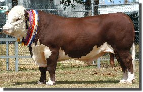
(c) http://yallaroo.murrayfrancis.com/

Herefords are massive, red and white colored animals. The head is usually entirely white and covered in curly, thick fur. Grows slower and gains fat faster than larger breeds.
Size (cows): 600-850 kg
Size (bulls): 1100-1300 kg

 Simmental is colored much like the Hereford, but the head is usually not entirely white. It is originally from the Simme Valley in Switzerland. It grows fast and generally gains fat slower than smaller breeds.

Size (cows): 700-950 kg

Size (bulls): 1200-1400 kg

Limousin  is another French beef cattle breed, and has originally been used as a working animal as well as for beef production. It has a high carcass percentage, i.e. the ratio between carcass weight and live weight. It grows fast and generally gains fat slower than smaller breeds.
Size (cows): 650-850 kg
Size (bulls): 1100-1300 kg

Carcass quality

Beef quality starts from carcass quality. A carcass is more valuable the less fat and bone is has, as the meat is the only economically important portion. The measurements are subjective, and based on the shape of the carcass. Most valuable cuts are evaluated especially carefully. In the European Union carcass quality is measured in an europ-scale: S > E > U > R > O > P (EEC  1208/81):

• S (superior) = All profiles extremely convex; exceptional muscle development (double-muscled carcase type)
• E (excellent) = All profiles convex to super-convex; exceptional muscle development
• U (Very good) = Profiles on the whole convex; very good muscle development
• R (Good) = Profiles on the whole straight; good muscle develop- ment
• O (Fair) = Profiles straight to concave; average muscle develop- ment
• P (Poor) = All profiles concave to very concave; poor muscle development

In addition to the EUROP-scale, the fatness of the carcass is evaluated from scale 1 (fat-free) to 5 (extremely fatty).

Two important concepts to consider are live weight and carcass weight. Live weight is the weight of the entire animal. Carcasss weight is live weight minus the weight of the head, genitalia, udder, digestive tract, internal organs, hide and hooves. The ratio between carcass weight and live weight is called carcass percentage. Carcass percentage varies between breeds, but is commonly 50-60 %.

When the carcass weight increases, to which the farmers often aim at, the relative proportion of lean meat decreases. In proportion, the amount of fat increases. The portion of the most valuable cuts (steak and filet) from the entire carcass does not change. Carcass weight can be increased by using plenty of concentrated feed, but a more effective method is to limit fattening by limiting energy intake at the finishing phase of the rearing.

Beef quality

Muscle becomes meat or beef after the animal has been slaughtered. Slaughtering causes chemical, physiological and biological changes in the muscle tissue. To prevent harmful changes, the animal and the meat must be handled correctly.

Beef quality consists of several factors:

• Physiochemical properties: pH, color, sarcomere length, run-off, consistency
• Chemical properties: Dry matter content, amount of protein, amount of fat
• Sensory properties: juiciness, flavor, tenderness

Meat becomes stringy and chewy when the myocine and actin filaments of the muscle stick together after death (rigor mortis). Usually carcases are cooled under +7 C before rigor mortis sets in, which causes the muscle to constrict due to cold. To prevent cold constriction the meat may be stimulated with electricity. Once the meat is cooked, the proteins break and the meat becomes tender.

Juiciness means the amount of muscle fluid which is released when the cooked meat is bitten into. It
is related to the amount of fat in the meat, since fat increases the water retention capacity. The largest part, 64-80 %, of beef is water. The water is retained between actin and myocin filaments. Water retention capacity decreases as the pH decreases after slaughtering. The pH of muscle is 7,2, but it drops to 5,6 within 24 hours after death. Fat percentage varies between 2-25 %. 

If the animal has little glycogen in its body right prior to slaughter, the meat does not develop enough lactic acid after slaughtering and the pH does not drop as fast and low as it should. This results in a tar meat, or DFD meat (dark, firm, dry). DFD meat is not used for whole-meat products because it has poor shelf life. 

Beef production: Basics

 Beef production is the production of beef and veal, i.e. the meat from cows, steers, bulls, heifers and calves. First we look at the differences between beef production to the production of other types of meat. Then we discuss the anatomy of meat, the growth of the beef animals and their carcass composition. The different methods of rearing beef cattle are discussed in later posts.

What is beef? Beef is the meat from bovines, that is "cows" of different age, gender and breed. The beef you see in a market comes either from beef production, milk production or from a combined farm with both milk and beef production. In Northern Europe, for instance, nearly 90 % of all beed originates from the dairy industry.

Compared with other animals reared for their meat, cows are relatively inefficient at transforming vegetation into meat protein. Dairy cows produce much protein and energy to their milk, but as meat producers they are even less efficient than beef cows.The chart on the left shows only the energy and protein in edible cuts. Energy in tallow, lard etc is not included.

One can also compare the animal species in terms of how well they utilize nitrogen. Feed N recovery efficiency in the edible weight fraction is defined as the percentage of the N in the animal feed that ends up in the edible portion of the animal. N recovery efficiency is low in beef production, only 8 %, but much higher for pork (~20%) and poultry (~30%). (Oenema et al. 2005)

Growth models and carcass composition

Growth can mean either the actual daily growth of an animal, the extra growth it puts on due to management and feeding, or the increase in edible cuts. For example: A calf grows 1500 grams a day (actual growth). Of  that, 400 grams is due to heavy feeding (extra growth). After the calf is slaughtered one can then calculate backwards how much of the 1500g went to the edible meat (increase in edible cuts).

Growth consists of four types of changes:

1. Changes in size (live weight)
2. Changes in appearance (height, diameter of chest...)
3. Changes in anatomical composition (fat percentage, ...)
4. Changes in chemical composition (chemical composition of muscles, fat etc)

Change in size, for example the weight, is an inaccurate measurement because it is affected by what the animal has eaten and drank. The weight of the digestive tract of a bovine varies tens of kilos during the day. The weight of a cow inceases most rapidly from birth until 6 months of age, when the growth slows and finally comes to an end at the age of 2-3 years. The model is very simplified, because bones, muscles, connective tissue and nerves have a very different rate of growth. This also affects the third measurement: the anatomical composition. First the animal gains mostly bones and nerves, then muscles and finally fat, all altering the anatomical composition of the carcass.

Daily growth is measured either as the proportion of daily growth to the live weight, i.e. 1500g / 250kg = 0,006 %, or simply as g/day. Final weight of beef breeds varies from 350 kg (a Dexter cow) to 1400 kg (Charolais bull). Bulls grow 10-20 % faster than steers (castrated bulls), while steers grow as fast as heifers (Galbraith and Topps 1982).

Changes in appeareance only describe how the different parts of the animal grow in proportion to one another. For example a calf has tall feet and a shallow chest, while a grown cow has shorter feet and very wide chest.

Chemical changes describe the changes in the composition of the body. The higher the live weight, the more fat there is in a kilo of carcass, and therefore also the relative energy content increases. At the same time the relative portion of crude protein decreases. As with all young animals, first to grow are the bones and nerve tissue, with muscles next and finally body fat. Breed and gender also affect the carcass composition. Steers gain 10-45 % more fat than bulls, and breeds like Angus and Hereford are fatter than for example Limousin and Charolais. Note that breed does NOT affect the composition of the lean (fatless) carcass.

All in all, the growth of an animal is summarized in the picture below (Rumsey 1991).

The anatomy of muscles

30-40 % of the live weight of a bovine consist of skeletal muscles. The quality of edible meat is affected by the chemical, biochemical and physiological qualities of the muscle both before and after slaughter. Growth, feeding, animal handling and meat processing after slaughter also all have an impact on the quality of the meat.For bovines, 30 largest muscles contribute 75 % of the weight of all the muscles. The largest muscle groups are in the pelvic limb (hind quarters) with 28,5 % of live weight, and neck/thorax with 22,4 %.

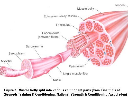
The anatomy of a skeletal muscle is shown in the picture to the left.The muscle is covered by epimysium, and consists of bundles of muscle fibres. The space between bundles is filled with perimysium, which has lots of nerves and blood vessels. Perimysium affects the tenderness of the meat. There is also fat between the muscle fibres, and this fat gives the meat it's marbling properties. Each muscle fibre is surrounded by endomysium, yet another type of membrane.



Each muscle fibre in the skeletal muscles has several nuclei. Fibres are surrounded by a sarcoplasm, which is a membrane, and sarcolemma, which is a type of elastic connective tissue. One fibre consists of 1000-2000 myofibrils. The functional unit of a myofibril is called a sarcomere. Sarcomere is where the muscle actually works, when thick and thin filaments of the sarcomere either slide closer or farther from a z disk (see the picture below). If the filaments become imbricated, the muscle constricts. When they slide farther apart, the muscle relaxes (returns to rest stage) or stretches. A very detailed video about the action potential and muscle activity can be found from Youtube.

Marbling and tenderness

Marbling of the meat means the increase of intramuscular fatty tissue, which occurs at the finishing phase of beef cattle rearing. Marbling is more pronounced with strong, grain-based feeding. The actual level of marbling is determined visually after slaughtering by estimating the percentage of fat in a cut of meat. Fat is seen as white areas in otherwise red meat.

The fat in the muscle is mostly based from de novo -fatty acid synthesis, which takes place in the rumen. The rumen biohydrogenates unsaturated fatty acids into saturated ones, so the fat of ruminating animals is more saturated than that of monogastric animals. For example, cattle have more saturated triglyceride 18:0 and less unsaturated 18:2 than pigs (Lawrence & Fowler: Growth of Farm Animals).

Tenderness is affected by the type of collagen in the perimysium, the connective tissue between bundles of muscle fibres. More important than types or the amount of collagen is cross-linking between the collagen types. Both the cross-linking and insolubility of collagen increase as the animal ages. That is why the meat from old animals is more stringent than the tender meat of young animals. However, when cooking meat in high temperatures even tender meat becomes stringent due to heat-induced chemical changes in the collagen.

Managing risk in animal breeding schemes

Animal breeding is not exact science in the sense that normally one cannot exactly predict the outcome, or even select the "ingredients". Each gamete (an egg cell or a sperm) is different, and their combination and further cellular divisions all include an effect of randomness. So each breeding scheme has risks. This post will address some of those risks and how to minimize their impact.

Inbreeding

Breeding always requires some inbreeding. This is because we want to increase the genes from one or few excellent animals, so we use them for males/females of several generations. Consider horse racing and show jumping: it's common to list the famous parents, siblings, half-sibs and grandparents of any horse to prove its value.

The change of inbreeding can be calculated as

ΔF= 1 / 2N_e

where N_e is the effective population size. If the pnumber of parents of different sexes isn't equal, then we estimate

ΔF ≈ (1 / 8N_m) + (1 / 8N_f)

Inbreeding works in two ways: inbreeding increases variance between lines/populations, but decreases variance among a line/population. Remember that inbreeding depression, the negative effect of inbreeding on genetic diversity, can be negated by breeding two animals of completely different lines.

Genomic selection versus progeny testing

Both agenomic selection schemes (GS) and progeny testing schemes (PT) have their own risks. Professors Alban Bucket  and Jarmo Juga from the University of Helsinki have studied the risks in bovines. They state that in GS schemes the rate of inbreeding is slightly higher than in PT schemes, but reciprocally the genetic response is much higher in GS than in PT. The choice becomes a matter of balancing the risks. How high of an inbreeding level do we accept to get strong genetic response? 

Bucket and Juga state that if the amount of sires is not increased, the risk is comparable between GS and PT schemes. The risk in GS can be further minimized by increasing the amount of MOET (multiple ovulation, embryo transfer) and the number of genotyped females.This increases the genetic diversity and allows effective Mendelian variance. However, increasing the amount of AI bulls in a GS scheme increases the risks of inbreeding.

Preserving genetic diversity

As has been stated earlier, selection and inbreeding impact genetic diversity in two ways: the variance between lines increases, while the variance within lines decreases. If a line equals a breed, the impact can be very strong.One example can be found from the study by Uimari and Tapio, who studied how the effective population size has changed over generations in two pig breeds. During 50 generations, selection has decreased the effective population size from 600 to a mere 50. The decrease is simply due to breeding selection.

The impact of selection to the Ne of two pig breeds.
(c) Uimari and Tapio

Maintaining genetic diversity should be duly considered in every breeding scheme. By genotyping a large amount of animals it is possible to ensure diversity by pairing unrelated animals. By genotyping one can also ensure that rare alleles stay in the population, and that there is enough heterozygozity. These two go often hand in hand: rare alleles are found most often in heterozygotes than in homozygotes. By genotyping one can also preserve traits of specific interest and genomically control the level of inbreeding.

FAO, The Food and Agriculture Organization, has created a simple chart about preserving genetic diversity. The chart is part of their publication considering The State of the Worlds ANGR for Food and Agriculture (ANGR = Animal genetic resources). It shows that the actions required are rather simple. Because really - 

all it takes is the courage to look beyond monetary gain and efficiency.

Calculating breeding values

Basics of animal breeding have been covered earlier in this blog. We've discussed the very basics of animal breeding as well as the  Mathematics of animal breeding . Optimization of animal breeding schemes has also been briefly considered. Today we take a closer look at calculating the breeding value using statistical concepts and information from various sources.

Estimated Breeding Value

When calculating EBV (estimated breeding value) for an animal, we usually want to combine information from various sources. We have results from the animal itself, but also from its relatives. However, EBV is always for one trait only.

The formula for an EBV is

 = b₁x₁ + b₂x₂ + ... b_nx_n

where  is the EBV, b1 is the regression coefficient for trait 1 and x1 is the result for trait 1. Seems simple, doesn't it? Now all we need to do is calculate the b values. The key to the b values is to remember where dealing with several bits of information at once, and every "bit" is actually an equation

 Â = (y1 - μ) = a₁ + e₁

where  is the EBV, y1 is the animal's own result in trait 1, μ is the population mean result in trait 1, a1 is the additive genetic effects contributing to the trait and e denotes the environmental factors contributing to the trait. Simply put: an EBV consists of genetics and environmental factors.

So, the b's must fulfill equations for traits 1 ... n at the same time. Instead of a group of equations we use matrices to calculate the b's. Only then can we continue to calculating the actual selection index. The matrix notation for calculating b's is

b = P^-1G

Here P and G are matrices. P includes the variances and covariances between phenotypic results. The marking P^-1 simply means that the transpose of the matrix P is used in the calculation. G is another matrix, which links the information sources to true breeding values. In the G matrix Ai denotes the true breeding value of animal i. Info1 and Info2 below are different information sources, for example animals 1 and 2.

You might remember that we never know the actual breeding value A, so we always work with the estimated BV, denoted as Â. However, with enough information and correct calculations it is assumed that A = Â. The trick in matrix G is to consider the genetic relationships between the information sources, here animals 1 and 2. If Info 1 is the animal itself, so that the source for info 1 = i, then Cov(Info 1, Ai) = Var(Ai). More generally,

Cov(Info x, Ay) = a(x,y) * Var(A)

and

Var(A) = h2 * s.d. (P)

where a(x,y) is the coefficient of genetic relationship between animals x and y. If x and y are full siblings, their coefficient of genetic relationship is 0,5, and Cov(Info x, Ay) = 0,5 Var(A). If they're half-sibs, it's Cov(Info x, Ay) = 0,25 Var(A) and so on. s.d. (P) is the standard deviation of the trait P, or the trait for which we are calculating the breeding value for. Standard deviation of P is the square root of the variance of P.

Selection index and economic breeding value

So now we can calculate the EBV for one trait. What if we want to combine several traits into one number? Then we need a selection index. It works like EBV, but combines information from several sources and several traits into one.

A selection index can either be optimal or common. The difference is in the coefficients: optimal coefficients minimize the variance between true breeding values and estimated breeding values. In a common selection index the coefficient b is said to be "any b₀", but in the optimal index b = P^-1Cv. The optimal index considers covariances, and breeding accuracies impact the b coefficients.

Here we can see a new matrix, C. C is used if the measured traits are not the same as the traits to be improved. For example, we might measure weight and thickness of back fat, but we want to improve weights and percentage of lean meat. Now we need the matrix C, which relates to the other matrices as shown in the picture below.

If we want to include money to the calculations, we get a total breeding value. Money is used in breeding values to give economical weights to each trait. This weight is entirely decided by animal breeders, and based on what they think is most important. Economical weight isn't linked to genetics or phenotype in any way. It is simply a way to put the traits into some order of importance.Often economical values is derived from actual profits or costs regarding the trait in question. The weight is currency per 1 unit of increase/decrease in the trait, for example euros per +- 1 kg of meat or dollars per +- 1 weaned piglet. The economical value can be used to ompare the costs and profits between different breeding schemes.

(c) Wikipedia Commons

For example:
We have two schemes for pig breeding. One scheme gives us - 0,5 piglets per sow, but 10 kg more meat since the surviving piglets are heavier. The other scheme gives + 0,7 piglets but -6 kg meat.  Let us assume that 1 kg of meat is +10 euros and 1 piglet is 15 euros.

Now the first scheme yields (-0,5 * 15) + (10*10) = 92,5 euros, and the second scheme (0,7 * 15) + (-6 * 10) = -49,5 euros. With these exaggerated numbers it is easy to see which scheme would be more profitable for the producer.

Economic weight can also be used when restricting a selection index. We may want to improve one trait, but leave another trait untouched. In that case the economic value of the trait, which is not allowed to change, is set to 0,

Total breeding value

Using indices and economic breeding values we can calculate a total breeding value for an animal. The formulas are

H = v'g

I = b'x where b = P^-1Gv

 H = total breeding value, estimated using the index I
v = economical weights of traits
g = breeding values of traits
I = selection index
b = regression coefficients for traits
x = vector of observations [result1    result2    resultn]
P = covariances and variances between observations
G = covariances and variances between traits to be improved and measured traits.

Additional information and sources

Mrode, R. A. Linear Models for the Prediction of Animal Breeding Values, 2nd edition. CABI Publishing, USA. ISBN-13: 978-085199-000-2

Cameron, N. D. Selection Indices and Prediction of Genetic Merit in Animal Breeding. CAB International, USA. ISBN-13: 978-085199-169-6

GenUp-software for playing with genetics: http://www-personal.une.edu.au/~bkinghor/genup.htm