Summary: Genetics, math and statistics

Variance components

Variance and variance analysis have been discussed earlier in this blog, so for now let's just remind ourselves that variance expresses the variation of the data: how far apart are the extreme values in the current dataset. Variance is also expressed in the same units than the data, so the unit affects the amount of variance (for example 1,5kg vs 1500g). 

Variance components are just the different factors that create variation between measurements. 

Variance components in animal breeding can be viewed from two perspectives: genetic vs environmental contribution (which together are the phenotypic variance), or dam/sire vs residual variance. Additive, maternal and dominance effects together form the genetic contribution. Common and general environment form the environmental contribution . Therefore

P = Var(A) + Var(M) + Var(D) + Var(e) + Var(eg).

All these contributions are built from variance from the dam, the sire and the residual. The chart below shows how the different components (pillars) are built. Note that sire variance (Var(s)) affects only additive genetic variance, of which it constitutes 25 %. Therefore Var(s) = 0,25 Var(A), and Var(A) = 4*Var(s). Dam variance is also 25 % of the additive genetic effect and dominance effect, but 100 % of common environmental and maternal effects.

Only some of the components above are inherited from parent to offspring. The rest are often ignored, so the formula can be simplified into

Var(P) = Var(A) + Var(M) + Var(e).

One interesting aspect about variation is that when the reliability of the breeding value, r_TI, increases, the variance of estimated breeding values increases as well. This is because the higher the reliability, the better we see the differences between the animals, and the more variation we get. However, when the reliability increases, the variance of the true breeding values decreases between animals with the same estimated breeding value. This is of course because the increased reliability brings our estimation closer to the true breeding value. One has to consider variance in its context.

Heritability h² is often written as additive genetic variance divided by phenotypic variance, i.e Var(A) / Var(P). Considering the previous formulas, heritability can be deduced from sire variance:  h² = 4 * (Var(s) / Var(P)).

Equations

Change of gene frequency under selection is

where q1 is the frequency of the selected gene after one generation, q is the square root of the original frequency (q2), s is the coefficient of selection and q2 is the original frequency as per the Hardy-Weinberg equation (q² + 2pq + p² = 1). 



Number of generations required

The number of generations required to achieve a certain breeding objective is calculated thusly:

where t is the number of generations, qt is the gene frequency after t generations and q₀ is the original gene frequency. q_t = q₀ / (1 + tq₀).



Coefficients

Coefficient of selection, s

Coefficient of selection is the proportionate reduction of gametic contribution of a genotype compared to the standard genotype. It shows how much less animals of a certain genotype, usually the less facorable, affect the next generation when selection takes place. For example how much less gametes do unpolled animals contribute compared to polled, when polled ones are selected for breeding.

The contribution of the favorable genotype is 1, the coefficient is s so the contribution of the less favorable genotype is 1-s.

If s = 0,1, then the contribution of the favorable genotype is 1 and the contribution (and the fitness) of the less favorable is 1-0,1 = 0.9. In practice, for each 100 zygotes by the favorable genotype, 90 zygotes are born by the less favorable.

Genetic analysis

XKCD's take on genetic analysis.

Genetic analysis may sound complicated, but it relies on very simple principles of heredity, statistics and probabilities. Sometimes the genotypes are not known at all, and we need to look at pedigrees to determine models of heritance. Here some basic principles of genetic analysis are discussed. Later on a post on bioinformatics will make a deeper analysis on how to analyze known genes an genomes.

Calculating probabilities

Inheritance, or which genes each parent passes on to the offspring, is always partially random. This is why probabilities are important. For example if we know the absolute frequency, i.e. the number, of a certain allele in a sample, we can deduce the probability of one randomly picked individual having that particular allele. Set the absolute frequency of the allele a to 118. Now we know that there are 118 a alleles in our sample of 500 chromosomes. The probability of a random individual to have a is simply the amount of a divided by the number of all possible alleles: 118 / 500 = 0,236. This is also the relative frequency of a.

So, the probability of A, whatever A is, is P(A) = the number of favorable results / the number of all possibilities. The probability of A's complement, of A not happening, is 1- P(A). Combinations of two or more independent variables are calculated as follows: P(A and B) = P(A) * P(B) and P(A or B) = P(A) + P(B). An example of a complement: if a chromosome has the allele a, it cannot have the allele A. Only either one or the other (barring some rare genetic mutations, which are not considered here).

The probability of two separate outcomes depends on if the outcomes are related or not. A union means that either (A or B) or (A and B) happen. For independent variables the union would be P(A) + P(B) - P(A u B). For dependent variables the union is zero: if A has happened, B cannot happen, or vice versa.

To ease your stress, here is a cute animal.

The conditional probability, the probability of A happening when we know that B has already happened and A and B are dependent, is (P(A) * P(B)) / P(B). This is often marked as P(A|B).

Permutations and combinations deal with the order of several possibilities. Permutations are used when the order of the events is important, and is counted as n!. Combinations take all orders into consideration, and are counted as n! / (r! (n-r!)).

Binomial probability is a bit more complex. It is used when we want to determine the probability of getting exactly r favorable results, each with the probability of p, out of n repeats. The magic word here is exactly - when that is used in an exercise, think of binomials.

 

More on probabilities:

Khan Academy

Wolfram

For the mathematically gifted: Wikipedia 

Cut the Knot (also covers Bayesian methods)

Statistics

Statistics have been covered before in a post named Variance Analysis (one of the most popular posts in this blog!), so I'll just remind you of the formulae we will need when doing genetic analysis.

There are thousands of helpful websites you can look up for more information on statistics. Here are just a few:

Khan Academy

x2 (khi squared) test and genotypes

x2 test and plant breeding

Statistics.com
Mendelian genetics by Phillip McLean

Examples

Right, let's get down to the real deal and do some analysis! The examples are from University lecture materials for course in genetic material, but I unfortunately cannot share the entire material due to copyright restrictions and a language barrier - the materials are not in English :)

Example 1. Parents are heterozygotic concerning their eye color. They both have the allele s for blue eyes and the allele S for brown eyes. Calculate the probability that they will have 

a) a child with blue eyes  b) five children with blue eyes.

From the way the alleles are written we see that S is the dominant allele. The genotypes of the parents are Ss and Ss, so the possible genotypes of their children are 

Now we can see that 3/4 of the offspring have the dominant allele, so only 1/4 has blue eyes (homozygote ss). Therefore the P(a child has blue eyes) is 1/4 = 25 %. The probability for each subsequent child is similar, so P (five of five children have blue eyes) is 0,25 * 0,25 * 0,25 * 0,25 * 0,25 = 0,000977.

Example 2. 32 % of people infected with a rare illness have mutation A, and 16 % have mutation B. 10 % of those infected have both A and B. Calculate the probability of randomly selected person to have at least one of the mutations? 

The selected person must now have either A or B or both. What is needed is the union of A and B: P(A) + P(B) - P(A u B) = 0,32 + 0,16 - 0,1 = 0,38. 38 % have either A, B or both mutations. Note that the union P(A u B) is NOT A*B in this case, but it is given as 10 %.

Example 3. There are 2 boys and 5 girls in a family. In how many different sequences could the children have been born? 

Because the order is not important, we'll use combinations: n over r, i.e. n! / r!(n-r)!. The n now is 7, the number of all kids. The r can be either 2 or 5: both give the same result. If r = 2, then 

7! / 2!(7-2)! = 7! / 2! 5! = 5040 / 240 = 21.

Example 4. Parents are heterozygotes concerning a rare recessive illness. Calculate the probability that out of three children

a) all are healthy

b) two are ill

c) at least two are ill.

a) Recessive heterozygotes produce 25 % of recessive homozygotic alleles (see example 1). The probability for each child to be healthy is thus 1 - 0,25. P(all are healthy) = 0,753 = 0,422.

b) Two out of three must be ill, so we need the binomial distribution. Now r = 2, n = 3 and p = 0,25. The first factorial, n over r, gives 3!/2!(3-2)! = 3. Continuing from there we have 3 * 0,25² * (1-0,25)^3-2 =3 * 0,0625 * 0,75 = 0,141.

c) If at least two must be ill, then the probability is P(two are ill) + P(three are ill). The first part is calculated like in part b: 3 * 0,25² * (1-0,25)^3-2 =3 * 0,0625 * 0,75 = 0,141. P(three are ill) is simply 0,253 = 0,015625. So P(at least two are ill) = 0,141 + 0,015625 = 0,156. 

Example 5. The penetrance of a certain illness varies between genotypes. The penetrances are 0,01 for AA, 0,05 for Aa and 0,5 for aa. In a population the allele frequencies are  f(a) = 0,05 and f(A) = 0,95. The population is in Hardy-Weinberg equilibrium. Count the prevalence of the illness in the whole population.

Whoa, lots of terms here! Penetrance is the probability of expressing a certain trait. Here the trait is the illness. H-W balance means that in an ideal population, where q and p are the relative frequences of a alleles, there are p² dominant homozygotes, 2pq heterozygotes and q² recessive homozygotes. What are they actually askingfor is the prevalence, i.e. the probability of a random member of the population to have the illness.

First we need to calculate the frequencies of the genotypes in the population. With the H-W equilibrium and the given frequencies we know that p = 0,05 and q = 0,95. Now the genotype frequencies are  
AA  = dominant homozygotes = p² = 0,95² = 0,9025
Aa = heterozygotes = 2pq = 2*0,95*0,05 = 0,095
aa = recessive homozygotes = q² = 0,05² = 0,0025

Now each genotype has its own probability of actually expressing the illness. To make it easier to understand we can build a table of  a tree of probabilities:

So now the random person we select has a 0,9025 % chance of having the genotype AA, and then 0,01 % chance of being sick.  Note that these variables are independent (a person can only have one genotype and be either sick or healthy). The possibility of expressing the illness is thus P(has a certain genotype) * P(is sick).

P(is sick) = P (AA and sick) + (P Aa and sick) + P(aa and sick) = P(0,9025 * 0,01) + P(0,095*0,05) + P(0,0025*0,5) = 0,009025 + 0,00475 + 0,00125 = 0,015.

Example 6. The observed genotype frequencies in a population are f(AA) = 31, f(Aa) = 89 and f(aa) = 122). Is the population in Hardy-Weinberg equilibrium?

If we were mean about it, we'd say no because no actual population is ever in H-W equilibrium. However in an exam we'd get 0 points for that, so let's calculate this. Now we need to use x2 or khi squared test. We already have the observed frequencies. Now we need the expected frequencies, i.e. the frequencies if the population was in H-W equilibrium.

To get there we calculate the allele frequencies in the population. There are 31 creatures with two A alleles and 89 with one. In total we then have 2 * 31 + 89 = 151 A-alleles. The recessive allele a is calculated similarly: 2*122 + 89 = 333. In total there are 151 + 333 alleles, so the relative frequencies are 151/484 = 0,312 for A and 1-0,312 = 0,688 for a. So now p = 0,312 and q = 0,688.The expected absolute genotype frequencies are now

AA  = p² = 0,3122 * 24² (the size of population) = 23.56
Aa = 2pq = 2 * 0.312 * 0.688 * 242 = 103.89
aa = q² = 0.688² * 242 = 114.55

We need to calculate the chi squared test value using the formula

To make it easier, let's put our values to a table. Then we can use the formula and calculate the x2 test variable.

The value 4.97 is not the answer. Remember the question: is the population in H-W equilibrium? The answer hides in a x2 distribution table. To use that we need degrees of freedom (df), which in an chi squared good of fit test is the number of classes minus 1. Here we have three classes (three genotypes), so our df = 3-2 = 1. Now we look at a x2 distribution table such as this.

With df = 2 we find that our  x2-value, 4.97, goes between 4.605 and 5.991. The corresponding P-values are 0.10 and 0.05. So our p is 0.1 - 0.05. Without going too far into interpreting p-values we can just note that it is higher than 0.05 which means that we abadon the hypothesis 0 (the population is in H-W equilibrium). P > 0,05 shows us that the population is NOT in H-W equilibrium.

Variance analysis

DISCLAIMER: Statistics is scary. To ease the stress caused by writing and reading about it, I've included cute pictures along the way. One way of making statistics less traumatizing is to use funny examples, pretty colors or banging your head with a hammer, which is probably less painful than calculating regression factors. However, if you do read this post and end up in an insane asylum, try to get the room 7. I've hidden a hammer under the pillow.
 
Statistics is the science of controlling uncertainty in measurements and estimations. It's not just about collecting data and turning it to fancy graphs, but to really ensure that the information is correct. The graphs are just the tip of the iceberg of formulaes, tests and hypotheses. This post offers short explanations on some of the basic concepts of statistics. For more information, see KhanAcademy's excellent 10-minute videos on statistics.

A completely irrelevant but cute bunny.


Statistics: A branch of mathematics dealing with the collection, analysis, interpretation, and presentation of masses of numerical data. A collection of quantitative data. A statistic would be a single term or datum in a collection of statistics, or a quantity (as the mean of a sample) that is computed from a sample.(Merriam-Webster Dictionary)

Median, mean and mode: When the numerical values of the data are arranged from smallest to largest, median is the value in the middle, or the mean of the middle values (if there are even number of results). Mean is the arithmetic mean of the values: the sum of the values divided by the number of values. Mode is the value which is represented most often in the set of data. For example, in a data set of
2  4  4  5  6  7  7  9
the median is the mean of the two values in the center ( (5+6)/2 = 5.5 ), 4 and 7 are modes and the mean is (2+4+4+5+6+7+7+9)/8 = 5.5. Note that median and mode are not always identical.

Population and sample: Population is the all past, present and future realizations of the values of the object to be measured. A population of soda cans would mean all of the cans which have been produced, are produced and will be produced in the future. Population statistics can only be estimated from a small proportion of the population, namely a sample. We select a decent amount of soda cans, measure them, and estimate how well those results might represent the whole population.

Different statistical values for a population and for a sample are sometimes calculated a bit differently. The denotations also differ. Thus it is clear when the statistics are about an observed sample or estimated for a population.

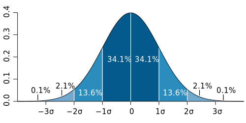
Normal distribution: The most common distribution of values, where middle-range observations are the most common, and extremely small and large observations are rare. Many natural traits, like height or IQ, are normally distributed, especially when a data set of over 30 observations is used. Normal distribution is in the shape of a Bell-curve. A really useful attribute in a normal distribution are that it's symmetrical around it's central peak:

(c) Wikipedia

Variance and standard deviation: Variance shows how far each value in the data set is from the mean.Variance is relative, and independent from the values in the data set. It doesn't measure the difference between the mean and extreme values, but the distance between them in units of standard deviation. Standard deviation is simply the square root of variance. Population variance is often denoted as sigma to the power of two (σ²), and standard deviation as sigma (σ). Sample variance is mu to the power of two (µ²), and sample standard deviation is mu (µ).

Statistical testing: Testing in statistics is rather depressing: it's about estimating the risk of being wrong. First the research hypotheses are formed, and then the actual data is collected. A  set of two or more subsamples (or subpopulations) are compared by using either parametric or non-parametric statistical tests. The aim is to estimate the risk of being wrong when the formulated H₀ (zero hypothesis) hypothesis is correct.

Variance? Is that something edible?
(c) redpandanetwork.org

H₀ is always a "nothing happens" hypothesis, and H₁ is it's opposite. Say that you've measured the weight of red pandas in two different regions in China. You calculate means, variances etc for the two samples (the two groups of pandas). Your H₀  must be that there's no difference in the weights. Your H₁ must then be either "There is difference in the weights", "the pandas in the area A are lighter" or "the pandas in the area A are heavier."




Variance analysis
 Variance analysis is a parametric test for comparing the mean of three or more subpopulations. The same comparation for two populations is done using a paired Student t-test. Variance analysis has three requirements:

1. The populations in variance analysis  must be normally distributed
2. Variances are equal in all subpopulations
3. The observations are independent (not depending on one another)

The populations may be of different size. Usually the populations in variance analysis are caused by different treatments to the studied unit. For example, pieces of meat are treated with different preservatives to find the most effective one, or the  results of different excercise programs are compared. Again the zero hypotheses is that the treatments have no effect to the results ( µ₁ = µ₂ = ... = µ_n)

The structure of variance analysis is

x_ij = µ + α_i + ε_ij

where μ = common mean
α_i = the effect of treatment i
ε_ij = random error, which is normally distributed N(0,σ)

The idea behind variance analysis is to trace the variation in the observed results into separate sources. Variation can be caused by the treatments, or by other factors (residual error). If the assumptions for variance analysis are true, residual error is normally distributed with the expected value of 0. The total variation of the observations around the mean can be divided into two sums of squares, SStreatments and SSerror. The sum of SStreatments and SSerror is SStotal. SStreatments is the sum of squares of the variation caused by the treatments. SSerror is the sum of squares of the residual error.

In the formula above,
x_ij = the j:th observation of the i:th treatment
n = number of observations in a treatment
k = number of treatments
x_i+ = sample mean in treatment i
x = sample mean of all observations


F-test
Once we've established the SStotal, it's time to use SStreatments and SSerror for estimating the population variance. The sums of squares must be divided by their degrees of freedom (df). For SStreatments df is k-1, and for SSerror it's kn-k. This gives us mean sums of squares. Finally the actual test value F is calculated:

MStreatments = SStreatments / k-1          MSerror = SSerror / nk-k

F = MStreatments / MSerror

The test value F is F-distributed with degrees of freedom k-1 and nk-k.  The larger F is, the stronger evidence it gives against the zero hypothesis. The critical values of F can be found from the F-sheet (such as this). The observed value of F is then used to find out the observed p (probability to get the observed results if H0 is true). If a test of significance gives a p-value lower than the significance level α, the null hypothesis is rejected. I.e if the observed p < chosen significance level, H0 is rejected.

More on variance analysis:
http://www.itl.nist.gov/div898/handbook/prc/section4/prc433.htm
http://www.terry.uga.edu/~pholmes/MARK5000/Classnotes2.pdf
http://en.wikipedia.org/wiki/Statistical_significance